Exploring the Ford GoBike Dataset: Uncovering Insights into Bike-Sharing in the San Francisco Bay Area
BLOG №7

Table of Contents:
- Preliminary Wrangling
- Univariate Exploration
- Bivariate Exploration
- Multivariate Exploration
- Conclusion
Introduction:
Preliminary Wrangling:
# Load the dataset
df = pd.read_csv("201902-fordgobike-tripdata.csv")
# Display the first few rows of the DataFrame
df.head(5)


# Display information about the dataset, including column names and data types
df.info()
 After careful consideration, I have decided to drop the rows with missing values in the member_birth_year and member_gender columns. These missing values account for a small proportion of the dataset, and I believe that maintaining accuracy in the analysis is crucial. By dropping these rows, I ensure that the remaining data used for analysis is complete and reliable.
# Drop rows with missing values in the specified columns
df.dropna(subset=['end_station_id', 'end_station_name', 'start_station_id', 'start_station_name'], inplace=True)
df.dropna(subset=['member_birth_year', 'member_gender'], inplace=True)
After careful consideration, I have decided to drop the rows with missing values in the member_birth_year and member_gender columns. These missing values account for a small proportion of the dataset, and I believe that maintaining accuracy in the analysis is crucial. By dropping these rows, I ensure that the remaining data used for analysis is complete and reliable.
# Drop rows with missing values in the specified columns
df.dropna(subset=['end_station_id', 'end_station_name', 'start_station_id', 'start_station_name'], inplace=True)
df.dropna(subset=['member_birth_year', 'member_gender'], inplace=True)
# Check for missing values in the dataset
print(df.isnull().sum())

Good now we don't have missing values, we can continue our job.
After dropping values, now I will start to get into the dataset by calling some functions


After dropping the missing values, I noticed that the summary statistics of the dataset have changed slightly. I expected this because the dropped rows had missing values in certain columns, which can affect calculations such as mean, standard deviation, and quartiles.
Although there are minor changes in the summary statistics, it is not a significant issue. Since the dropped rows represent a small portion of the total dataset, the impact on the overall analysis is minimal. The remaining data still provides valuable insights and can be used for meaningful analysis.
I made the decision to drop missing values in order to ensure the accuracy and integrity of my analysis. By removing incomplete or unreliable data points, I can focus on a more complete and representative subset of the dataset, which leads to more reliable conclusions and insights.
Overall, I believe that the slight changes in the summary statistics after dropping missing values are acceptable and do not compromise the validity of my analysis.
From the table above, duration_sec and member_birth_year are important.

We convert the 'start_time' and 'end_time' columns to the datetime data type using the pd.to_datetime() function. This will allow us to easily work with time-related data and perform various time-based operations.
# Convert 'start_time' and 'end_time' columns to datetime
df['start_time'] = pd.to_datetime(df['start_time'])
df['end_time'] = pd.to_datetime(df['end_time'])
We convert the start_station_id and nd_station_idcolumns to the int64 data type using the astype() method. This change was made because station IDs are typically represented as integers, and using the int64 data type allows for more efficient storage and supports integer-based operations.
# Convert 'start_station_id' and 'end_station_id' columns to int
df['start_station_id'] = df['start_station_id'].astype(int)
df['end_station_id'] = df['end_station_id'].astype(int)- Printing the unique values in the
user_type column allows us to see the different types of users in the bike-sharing system. - Printing the unique values in the
member_gender column helps us understand the distribution of gender among the users. - Printing the unique values in the
bike_share_for_all_trip column provides insights into whether users share bikes for all their trips or not.
# Looping through columns to print unique values
columns = ['user_type', 'member_gender', 'bike_share_for_all_trip']
for column in columns:
print(df[column].unique())
This code will provide the count of unique values in the user_type column, which helps in understanding the proportion of subscribers and customers in the bike-sharing system.
# Get the count of each unique value in the 'user_type' column
print(df['user_type'].value_counts())
 You can see that subscribers are ten times bigger than customers
This code will display the count of unique values in the member_gender column, giving insights into the gender distribution among the users. It helps identify the dominant gender among the users.
# Display the count of each unique value in the 'member_gender' column-->
print(df['member_gender'].value_counts())

Indeed, from the available data, it appears that there is a higher proportion of male users compared to female and other genders in the bike-sharing system in the San Francisco Bay area. The count of male users is significantly higher (130,500) compared to female users (40,805) and users with other genders (3,647). This suggests that the bike-sharing system is more popular among male riders.
By using this code, we can get the count of unique values in the bike_share_for_all_trip column. It helps determine the frequency of users who share their bikes for the entire trip ('Yes') compared to those who don't ('No').# Show the count of each unique value in the 'bike_share_for_all_trip' column
print(df['bike_share_for_all_trip'].value_counts())

# Define the function to print value counts
def print_value_counts(column):
    value_counts = df[column].value_counts()
    print(value_counts)

# Print value counts of the 'start_station_id' column
print("Value counts of the 'start_station_id' column")
print_value_counts('start_station_id')
print("\n")

# Print value counts of the 'end_station_id' column
print("Value counts of the 'end_station_id' column")
print_value_counts('end_station_id')
print("\n")

# Print value counts of the 'start_station_name' column
print("Value counts of the 'start_station_name' column")
print_value_counts('start_station_name')
print("\n")

# Print value counts of the 'end_station_name' column
print("Value counts of the 'end_station_name' column")
print_value_counts('end_station_name')
print("\n")


What is the structure of the dataset? Dataset Structure
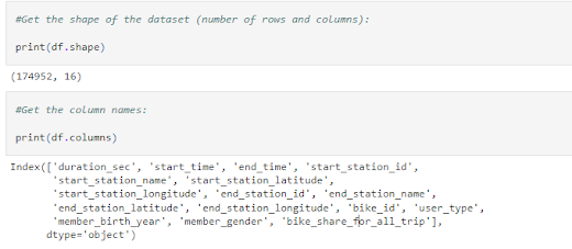
After dropping the missing values, the dataset now consists of 174,952 rows and 16 columns. Each row represents an individual ride made in the bike-sharing system covering the greater San Francisco Bay area. The dataset includes the following columns:
duration_sec: The duration of the ride in seconds (numeric)start_time: The start time of the ride (datetime)end_time: The end time of the ride (datetime)start_station_id: The ID of the start station (numeric)start_station_name: The name of the start station (string)start_station_latitude: The latitude of the start station (numeric)start_station_longitude: The longitude of the start station (numeric)end_station_id: The ID of the end station (numeric)end_station_name: The name of the end station (string)end_station_latitude: The latitude of the end station (numeric)end_station_longitude: The longitude of the end station (numeric)bike_id: The ID of the bike used for the ride (numeric)user_type: The type of user (either "Customer" or "Subscriber")member_birth_year: The birth year of the user (numeric)member_gender: The gender of the user (either "Male", "Female", or "Other")bike_share_for_all_trip: Indicates whether the user shared the bike for the entire trip (either "Yes" or "No")
This structure provides an overview of the columns and their respective data types, which will be helpful for analyzing and visualizing the data.
What are the main features of interest in my dataset?Main Features of Interest
From my perspective, the main features of interest in the dataset are as follows:
Start Station ID and Name: The unique values in the
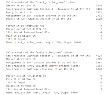
start_station_idandstart_station_namecolumns provide insights into the starting point of the bike rides. By examining the count of unique values in these columns, we can identify the most frequently used start stations. For example, the station with ID 58 has the highest count of 3,649 rides, followed by station 67 with 3,408 rides. Understanding popular start-stations helps in analyzing user preferences and planning station infrastructure.End Station ID and Name: Similarly, the unique values in the
end_station_idandend_station_namecolumns give us information about the destination of the bike rides. By analyzing the count of unique values, we can identify the most commonly used end stations. For instance, the station with ID 67 has the highest count of 4,624 rides, followed by station 58 with 3,709 rides. This helps us understand popular destinations and can be useful for station planning and optimizing bike availability.User Type: The unique values in the
user_typecolumn provides insights into the types of users in the bike-sharing system. By examining the count of unique values, we can determine the proportion of subscribers and customers. In our dataset, there are 158,386 subscribers and 16,566 customers. This information helps us understand the user base and tailor services accordingly.Member Gender: The unique values in the
member_gendercolumn gives insights into the gender distribution among the users. By analyzing the count of unique values, we find that there are 130,500 male users, 40,805 female users, and 3,647 users of other genders. Understanding gender distribution helps in designing targeted marketing campaigns and identifying any gender-based patterns or preferences.Bike Share for All Trip: The unique values in the
bike_share_for_all_tripcolumn provides insights into whether users share their bikes for the entire trip or not. By examining the count of unique values, we find that the majority of users (157,606) do not share their bikes for the entire trip, while a smaller portion (17,346) do. This information helps in understanding the level of bike sharing and its impact on trip durations and bike availability.
These features provide insights into the usage patterns, popular routes, user preferences, and demographic distribution within the bike-sharing system. Analyzing start and end stations helps in identifying demand patterns, optimizing station locations, and improving the overall user experience. Additionally, understanding user types, gender distribution, and bike-sharing behavior helps in tailoring services and marketing strategies to meet user needs and preferences.
Univariate Exploration:
Question 1: What is the distribution of ride durations?

Observation:
The histogram shows the distribution of ride durations in seconds. Most rides have durations between 0 and 2000-4000 seconds, with the peak around 450-700 seconds. There are only a few rides with longer durations, indicating that the majority of rides are relatively short.
Question 2: How does the number of rides vary across different user types?

Observation:
The bar plot displays the number of rides recorded for each user type. Subscribers have a significantly higher number of rides compared to customers. This suggests that the bike-sharing system has a large base of subscribers who use it more frequently.
Question 3: What is the proportion of customers and subscribers?

Observation:
The pie chart illustrates the proportion of user types in the bike-sharing system. Subscribers make up the majority, accounting for 90.5% of the users, while customers represent the remaining 9.5%.
Question 4: Which start stations are the most popular?

Observation:
The bar plot displays the top 10 most popular start stations based on the number of rides. Market St at 10th St is the most popular start station, followed by San Francisco Caltrain Station 2 and Berry St at 4th St.
Question 5: Which end stations are the most popular?

Observation:
The visualization displays the top 10 popular end stations in the bike-sharing system. The bar plot provides insights into the frequency of usage for each end station. Based on the number of rides, we can determine the popularity of different end stations. The station with the highest count, "San Francisco Caltrain Station 2 (Townsend St at 4th St)," is the most frequently used end station, followed by "Market St at 10th St" and "Montgomery St BART Station (Market St at 2nd St)." These stations serve as popular destinations for bike rides, indicating high demand and usage.
Question 6: What is the distribution of member genders in the dataset?

Observation:
The count plot illustrates the number of rides recorded for each member's gender. The dataset contains a significantly higher number of male users compared to females and other genders. This indicates a gender imbalance in the bike-sharing system, with males being the predominant users.
Question 7: What is the distribution of bike-sharing behavior (bike_share_for_all_trip)?

Observation:
The count plot showcases the number of rides based on the bike-sharing behavior of users. The majority of users do not share their bikes for the entire trip, while a smaller portion engages in bike sharing. This suggests that bike sharing is not a widespread practice among the users in the bike-sharing system.
Question 8: How many users share bikes for the entire trip?

Observation:
From the pie chart, we can observe the following:
- Approximately 9.9% of the users share bikes for the entire trip, as indicated by the "Yes" slice.
- The majority of users (90.1%) do not share bikes for the entire trip, as shown by the "No" slice.
- The chart highlights the difference between the two bike-sharing behaviors, making it easy to understand the proportion of users who choose to share bikes for the entire trip.
Question 9: What is the distribution of member birth years?

Observation:
The histogram represents the distribution of member birth years. The majority of users have birth years between 1980 and 2000, with the highest frequency observed around the late 1980s to early 1990s.
Question 10: How does the number of rides vary across different days of the week?

Observation:
The bar plot displays the number of rides recorded for each day of the week. We can observe that weekdays (Monday to Friday) have higher ride counts compared to weekends (Saturday and Sunday). The highest number of rides is recorded on Thursdays, while the lowest number is on Saturdays.
Question 11: How does the number of rides vary across different months of the year?

Observation:
The dataset only contains data for February, it means that there is no variation across different months, and visualizing the number of rides by month may not provide meaningful insights.
Bivariate Exploration:
Question 12: What is the relationship between the user type and the ride duration?

Observation:
The box plot visualizes the relationship between the user type and the ride duration. Here are the observations:
Subscribers: The box plot for subscribers shows a relatively narrower and lower box compared to customers. The median ride duration for subscribers is around 500 seconds (approximately 8 minutes). The lower and upper quartiles indicate that the majority of ride durations for subscribers fall within the range of approximately 300 to 800 seconds (5 to 13 minutes).
Customers: The box plot for customers displays a wider and higher box compared to subscribers. The median ride duration for customers is around 800 seconds (approximately 13 minutes). The lower and upper quartiles suggest that the ride durations for customers are more varied, ranging from approximately 500 to 1400 seconds (8 to 23 minutes).
Question 13: How does the ride duration vary between different genders?

Observation:
The violin plot illustrates the variation in ride duration between different member genders. Here are the observations:
Male: The violin plot for males shows a relatively wider distribution compared to females and other genders. The majority of ride durations for males are concentrated around the range of approximately 300 to 1200 seconds (5 to 20 minutes). The peak of the distribution is slightly skewed towards shorter ride durations, indicating that males tend to have shorter trips on average.
Female: The violin plot for females displays a narrower distribution compared to males. The ride durations for females are concentrated around the range of approximately 400 to 1000 seconds (7 to 17 minutes). The distribution is more symmetrical, with a slightly higher peak at the median ride duration, suggesting a more consistent pattern of ride durations.
Other Genders: The violin plot for other genders shows a distribution similar to that of females, with ride durations concentrated around the range of approximately 400 to 1000 seconds (7 to 17 minutes). The distribution is relatively narrower compared to males, indicating a more consistent pattern of ride durations.
Insight
To conclude for this visualization, the violin plot highlights the variation in ride durations between different member genders. While males tend to have a wider range of ride durations, females and other genders exhibit more consistent patterns with narrower distributions. These findings suggest potential differences in riding behavior and trip purposes among different member genders.
Question 14: Is there a relationship between the top 10 start stations and the user type?

Observation:
The stacked bar plot visualizes the relationship between the top 10 start stations and user types. Here are the observations:
Market St at 10th St: The majority of rides from this start station are by subscribers, indicating that it is a popular choice among regular users of the bike-sharing system. The number of customer rides is relatively lower in comparison.
San Francisco Caltrain Station 2 (Townsend St at 4th St): Similar to the previous start station, subscribers make up the majority of rides, suggesting a preference among regular users. The number of customer rides is relatively lower.
Insight
The stacked bar plot provides insights into the user type distribution for the top 10 start stations. Subscribers are the predominant user type for most of the popular start stations, indicating a strong base of regular users in these areas. The number of customer rides is relatively lower, suggesting that these start stations are preferred by subscribers who use the bike-sharing system more frequently.
Question 15: Are there any relationships between the start day of the week, user type, and the duration of rides?

Observation:
The box plot visualizes the relationship between the start day of the week, user type, and the duration of rides. Here are the observations:
Overall, the box plot reveals that ride durations are influenced by both the start day of the week and the user type. Subscribers tend to have shorter and more consistent ride durations, while customers have longer and more variable ride durations. Weekends (Saturday and Sunday) exhibit slightly longer ride durations for both user types, possibly due to different usage patterns and leisurely rides during weekends.
Multivariate Exploration:
Question 16: How does the ride duration vary across different user types and member genders?

Observation:
The heatmap visualizes the mean ride duration across different user types and member genders. Here are the observations:
-Male subscribers have the shortest average ride duration, followed by female subscribers. Other customers have the longest average ride duration among all categories.
-The shortest ride durations are observed for male subscribers, with an average duration of around 616 seconds (10 minutes). Female subscribers have slightly longer average ride durations of approximately 696 seconds (12 minutes). Other customers have the longest average ride duration, exceeding 1602 seconds (26 minutes).
-There is a clear distinction in ride duration between subscribers and customers within each member's gender category. Subscribers tend to have shorter average ride durations compared to customers, regardless of their gender.
-The heatmap provides a comprehensive overview of the ride duration patterns across different user types and member genders, allowing for easy comparison and identification of trends.
Insight:
The findings suggest that the combination of user type and member gender plays a role in ride duration. While males generally have shorter average ride durations compared to females, the distinction between subscribers and customers within each gender category is more pronounced. Subscribers, regardless of their gender, have shorter average ride durations, indicating that they may use the bike-sharing system for more frequent and shorter trips, possibly for commuting or regular transportation purposes. On the other hand, other customers tend to have longer average ride durations, indicating a different usage pattern, potentially for leisure or recreational purposes.
Question 17: How does the ride duration vary across different user types, the day of the week?

Observation:
The point plot visualizes the ride duration across different combinations of user types, the day of the week, and member genders. Here are the observations:
For both subscribers and customers, ride durations are generally longer on weekends (Saturday and Sunday) compared to weekdays.
Insight:
The findings suggest that the combination of user type, and the day of the week influences ride durations. Weekends tend to have longer ride durations compared to weekdays for both subscribers and customers, indicating potential differences in usage patterns and trip purposes.
Question 18: How does the ride duration vary between different user types, genders, and bike-sharing behaviors?

Observation:
The box plot matrix visualizes the relationship between ride duration, user type, member gender, and bike-sharing behavior. Here are the observations for each subplot:
Subplot 1: Ride duration by user type and member gender
For both subscribers and customers, females tend to have slightly longer ride durations compared to males and other genders. The difference in ride durations between genders is more noticeable among subscribers.
Subplot 2: Ride duration by user type and bike-sharing behavior
Subscribers who do not share bikes for the entire trip tend to have shorter ride durations compared to subscribers who do share bikes.
Subplot 3: Ride duration by member gender and bike-sharing behavior
Males and females who do not share bikes for the entire trip have similar ride durations. However, among those who share bikes, females tend to have slightly longer ride durations compared to males.
Subplot 4: Ride duration by user type, member gender, and bike-sharing behavior
Among both customers and subscribers, females who share bikes for the entire trip have the longest ride durations, followed by other genders who share bikes.
Subscribers who do not share bikes for the entire trip have shorter and less variable ride durations, regardless of the member's gender.
Conclusion:
Throughout my data exploration, I gained valuable insights into the bike-sharing dataset, examining various aspects such as univariate distributions, relationships between variables, and multivariate interactions. Here are the key findings and reflections from my exploration:
User Type Distribution:I observed that the majority of users in the dataset were subscribers, indicating a strong base of regular users who potentially use the bike-sharing system for commuting or regular transportation purposes. On the other hand, customers represented a smaller portion of the user base, suggesting that they may be more casual or occasional users of the system.Ride Duration:I found interesting patterns in ride durations. Subscribers tended to have shorter ride durations compared to customers, which aligns with the assumption that subscribers might use the system more frequently for shorter trips. As for customers, they had longer and more variable ride durations, suggesting a different usage pattern, potentially for leisure or recreational purposes.Gender Differences:I observed slight variations in ride durations between different member genders. Females tended to have slightly longer ride durations compared to males, indicating potential differences in riding behavior and trip purposes. However, it's important to note that the differences between genders were relatively small and not as prominent as the differences observed between user types.Start Station Analysis:By exploring the top 10 start stations, I found that subscribers were the dominant user type for the most popular start stations. This suggests a strong base of regular users in those areas, while customers represented a smaller portion of rides. This finding indicates that these start stations are preferred by subscribers who use the bike-sharing system more frequently.Day of the Week Analysis:I observed that the day of the week played a role in ride durations. Generally, ride durations were longer on weekends (Saturday and Sunday) compared to weekdays for both subscribers and customers. This trend suggests potential differences in usage patterns and trip purposes on weekends, possibly related to leisure or recreational activities.Multivariate Exploration:Through my multivariate exploration, I uncovered more complex relationships between variables. I observed interactions between user type, member gender, and ride duration, highlighting the importance of considering multiple factors simultaneously. The analysis also revealed interesting interactions between user type, the day of the week, and ride duration, providing insights into how riding behavior varies across different user types and days of the week.
In conclusion, this exploratory data analysis provided me with valuable insights into the bike-sharing dataset. I gained a better understanding of user types, ride durations, gender differences, and the influence of factors such as start stations and the day of the week on ride patterns.


Comments
Post a Comment